Home   >  Sample Problems   >   Laminar Flow Past a Cylinder

 

Laminar Flow past a Cylinder

 

A very common geometry in fluids engineering is the crossflow of a stream at velocity U_∞ past a circular cylinder of radius R. For plane inviscid flow, the solution superimposes a uniform stream with a line doublet and is given in polar coordinates by

 

 

At the surface of the cylinder, where r = R, we have u_r = 0 and u_q = -2 U_∞sinq, violating the no-slip condition imposed by intermolecular forces between the fluid and the solid at a low Mach number. From the above equations, the pressure distribution at the cylinder surface can be found from Bernoulli’s equation. The value of the coefficient of pressure, C_p, is

 

 

Integration of the inviscid C_p around the cylinder results in a value of zero for the drag, showing the inadequacy of the inviscid solution to represent the flow. The effect of viscosity is important. Physical observation of the flow past the cylinder shows that separation occurs in the rear surface. In addition, the flow is not symmetric in the wake region and pairs of vortices called Kármán vortex streets are developed and are convected from this region. Kármán vortex streets are caused by alternation of stable configurations for vortex pairs. Experimental measurements are available for this flow and the current calculations are compared with the inviscid solution as well as experimental measurements of the coefficient of pressure, C_p, drag, and lift coefficients.

 

 

Computational Procedure

 

A Mach number of 0.1 and a Reynolds number of 100 was chosen for the simulation.  The diameter of the cylinder is 1.0 and 197 ´ 144 ´ 3 grid points are used to solve the flow in a single block domain. The simulation type is simple CFD. The compact scheme is used for spatial differencing and Beam-Warming scheme is used for time differencing. The problem is solved as though two-dimensional in i and j directions. (Note that, although no spatial differencing is done in the k-direction, three grid points are still required in this direction, as this is the minimum number of grid points allowed in any direction.)

 

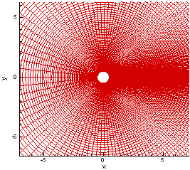
The computational mesh is set up with graded elements close to the wall in the normal direction. The computational mesh is shown in Figure P3.1(a). The initial conditions are as follows:

 

 

Obtain the Files

 

Both mesh files and project input files can be accessed below. Remember to place the grid files in a subfolder with the set up file /cylinder.

Setup file (cylinder.afl)

Grid file (cylinder.in).

 

Start the Simulation

 

Change the directory to the subfolder with the set up file. Start the simulation by

 

mpirun –np 1 mpiaeroflo.exe< cylinder.afl

 

 

Results

 

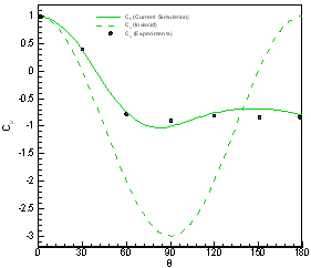
Steady-state results were obtained after the non-dimensional time reached approximately 130. Figure P3.1(a) is a close-up of the mesh of the computational domain. The mesh shows grading close to the surface of the cylinder, as well as in the wake region. Figure P3.1(b) shows the coefficient of pressure C_p compared with experiments and the inviscid theory. The results show agreement within 4% of the experimental values.

 

(a)                                                                                                                                        (b)

Figure P3.1 (a) Mesh of the computational domain, (b) Calculated coefficient of pressure compared with experiments and inviscid theory

 

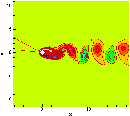
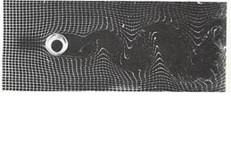
The vorticity plot is presented in Figure P3.2(a) showing the Kármán vortex streets. Figure P3.2(b) shows the vortex streets as streaklines from experiments presented in the source. A shedding frequency associated with the vortex street may be used to calculate the Strouhal number.

         

(a)

Figure P3.2 (a) Vortex street downstream of circular cylinder, (b) Vortex street from source, experimental timelines and streaklines at Re = 170

 

Figure P3.3 shows the lift coefficient as a function of time. The influence of the shedding on the lift is the cyclic variation observed in the plot. The maximum value of the lift coefficient is calculated to be 0.34. The period of the variation is 6.1375 which equal a Strouhal number of 0.163 compared with measured values of approximately 0.2 presented in the source.

 

The drag coefficient was obtained by integrating the coefficient of pressure. The result is a maximum value of 1.33 compared with a measured value of 1.4 presented in the source.

 

 

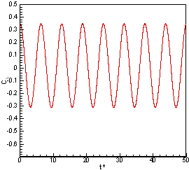
Figure P3.3 Periodic variation of the lift coefficient

 

 

References:

White, F. M., “Viscous Fluid Flow”, 2^nd Ed., McGraw-Hill, 1991. pp 8-11.